Offline Signature Verification

Demo site

Source Code

Skip to Result

Project Overview

This project utilises EfficientNetV2 ¹ as the feature extraction backbone and is complemented with a custom loss function inspired from Hard negative examples are hard, but useful², $L_{SC+}$. This project also utilises an extended version of the conventional $PK$ sampling technique, $PKFM$.

All of these choices were made according to existing research and reading materials. This project was made to address known limitations and challenges of utilising deep learning models in offline signature verification.

Challenges in this domain

• High intra-class variability
• High inter-class similarity
• Poor computational efficiency
• Imbalance of real-world training data

The primary objective of this project is to improve intra-class generalisability while ensuring skilled forgeries’ discriminatory ability remains strong.

Out of Scope

1. Digitally drawn signatures
2. Electronic Signatures
3. Non-Latin languages
4. Accuracy when poor quality images are used
5. Writer dependent verification
6. Signature extraction

Oversight

Like all models placed in critical systems, they can sometimes make potentially disastrous mistakes and require human oversight.

Problems

To the best of my knowledge, albeit admittedly limited, offline signature verification are still primarily driven by manual work. (I was informed of this during my internship)

Unlike machines, humans can’t operate on high volumes of documents at high speed over a long, continuous period of time. Since signatures are still used in important documents, particularly in financial, legal, and administrative contexts, errors are very often unacceptable.

Deep learning approaches often struggle with high intra-class variability and highly similar skilled forgeries. To deal with this, a lot of approaches cheat by implementing additional methods or models on top of their existing deep learning architecture and pipeline. This is not to fault the authors, but I do believe that there are still more optimisation that we have yet to implement.

If developers aren’t careful enough, OSV models that utilise the conventional triplet loss approach ³ can suffer from poor optimisation, wasting resources; most of the time ², the positive samples are already closer to the anchors than the negatives, leading to over-optimisation of anchor-positive pairs and causing poor generalisability towards intra-class signatures.

Approach

Pre-Processing Images

TLDR

RGB format is unnecessary

Binary format was opted for and it was achieved with Otsu’s thresholding

What we primarily want from the signature images are the strokes; thus, colours don’t play much of a role. RGB format would only provide irrelevant colour information, increasing computation power and possibly interfering with the model’s ability to extract relevant feature embeddings. On the contrary, grasyscale or binary format forces the model to focus solely on the strokes of the signatures by enhancing the contrast between the foreground and the background. It also minimises paper artefacts, reducing noise in each image.

Although greyscale format reduces unnecessary information, it may make the foreground less discernible from the background. To make the strokes pop out, I went with Otsu’s binarisation technique ⁴. This techinque automatically determines the optimal global threshold needed to convert the grayscale image into a binary image.

For example ⁵,

Before	After

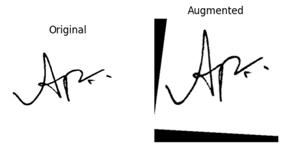
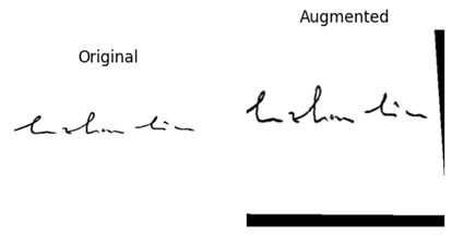
Unfortunately, I couldn’t solve the issue of lacking signature images that plagues this domain; however, this glaring issue may be mitigated by artificially boosting the number of training samples with data augmentation - resizing, rotation, scaling, and translation.

Example 1	Example 2

Code Snippet

TRAIN_TRANSFORM = transforms.Compose([
       transforms.Resize((384, 384)),
       transforms.RandomAffine(
           degrees=(-5, 5), 
           translate=(0.1, 0.1), 
           scale=(0.95, 1.05), 
           shear=(-5, 5)
       ),
 
       transforms.RandomResizedCrop(
           (384, 384), 
           scale=(0.9, 1.05), 
           ratio=(0.95, 1.05), 
           antialias=True
       ),
       transforms.ToTensor(),
       transforms.Normalize(
           mean=[0.5], std=[0.5]
   )])
 
TEST_TRANSFORM = transforms.Compose([
       transforms.Resize((384, 384)),
       transforms.ToTensor(),
       transforms.Normalize(
           mean=[0.5], std=[0.5]
   )]) 

Backbone

Training a CNN model from scratch would require tens of thousands to millions of examples to reach a satisfactory accuracy. It would also require extensive compute power, something that I don’t possess. Fortunately, I leverage existing state-of-the-art models via transfer learning to speed up the training process while ensuring satisfactory accuracy.

PyTorch offers A LOT of pretrained CNN models ⁶

Pretrained Models

- AlexNet
- ConvNeXt
- DenseNet
- EfficientNet
- EfficientNetV2
- GoogLeNet
- Inception V3
- MaxVit
- MNASNet
- MobileNet V2
- MobileNet V3
- RegNet
- ResNet
- ResNeXt
- ShuffleNet V2
- SqueezeNet
- SwinTransformer
- VGG
- VisionTransformer
- Wide ResNet

After doing some reading ^{1 7}, EfficientNetV2 was the top pick. The model improved upon EfficientNetV1, balancing computation efficiency with performance - this model performs $11\times$ faster while being $6.8\times$ smaller. Amongst the three available EfficientNetV2 variants, the mid-size variant offers the strongest balance between computation cost and performance; the largest variant contains more than twice the parameters of the mid-variant, yet it yielded only marginally better performance on ImageNet ¹.

Models	Top-1 Accuracy (%)	Parameters
EfficientNetV2-S	83.9	22M
EfficientNetV2-M	85.1	54M
EfficientNetV2-L	85.7	120M

I removed the classification head and replaced it with project layers that reduce the feature vectors to 256 dimensions.

Why 256?

Short answer:

It’s a nice middle ground

Long answer:

A 256-dimension offers a rich yet efficient feature space for encoding patterns. Since signature images are relatively simple, there is no need for a higher level of dimensions, as a higher dimension can lead to redundancy.

Loss Function

Triplet Loss

The conventional loss function is as follows:

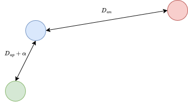
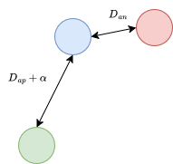
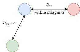
1. There are three nodes, collectively called a triplet, comprising an anchor, a genuine signature (positive), and a forged signature or an inter-class signature (negative).
2. The goal is to pull similar images (anchor and positive) closer while pushing dissimilar images (anchor and negative) away.
   • This is achieved by ensuring that the anchor is slower to the positive than it is to the negative by at least a margin ($\alpha$)

$$\begin{array}{r}{D}_{ap}+\alpha <D_{an}\end{array}$$

However, the triplets generated may have already satisfied this condition, slowing down convergence if these triplets are still passed through the network. To address this, the authors behind Hard negative examples are hard, but useful ² introduced online triplet mining to dynamically compute the triplets as training progresses. They achieved this by constructing large mini-batches that contain multiple examples per identity, selecting anchor-positive pairs from within the batch, and then dynamically identifying negatives.

• For hard triplets, the negative is chosen as the closest impostor to the anchor.
• For semi-hard triplets, the negative is farther than the positive but still lies within the margin.

Hard Triplet	Semi Hard Triplet

This paper is particularly important as it shows that this loss function is ideal for verification problems involving negative samples. Their online mining approach also led to countless inspirations down the line.

I decided to implement this loss function in conjunction to the custom loss function that I will be implementing.

$L_{SC}+$

This loss function is an extension of Hard negative examples are hard, but useful²

The authors of Hard negative examples are hard, but useful noticed that the conventional triplet loss function exhibits a couple of issues: poor optimisation and gradient entanglement. They proposed to simply ignore anchor-positive pairs and easy negatives to focus solely on penalising hard negatives.

Theoretically, this approach works well in the domain of offline signature verification; the high intra-class variation requires the model to have some degree of generalisability while maintaining a robust discriminatory ability.

However, there is a subtle failure if I just drag-and-drop their implementation. By removing the explicit constraint on anchor-positive similarity, the model is no longer encouraged to keep genuine signatures close together; over time, genuine embeddings can drift apart. In practice, this can lead to a higher count of false negatives: a genuine signature sampled later may fall outside of the verification threshold, although it belongs to the same user.

To mitigate this, I introduced a lightweight positive constraint that softly enforces intra-class cohesion while retaining the hard-negative emphasis. This lets me utilise the benefits of the existing loss function while preventing genuine signatures from drifting too far apart.

$$\begin{array}{r}{L}_{SC+}=L_{SC}(S_{ap},S_{an})+\mu L_{\text{pull}}\end{array}$$

Where:

• $L_{SC}$ is Selectively Contrastive Triplet Loss
• $L_{\text{pull}}$ is Positive Pull Regularisation
• $\mu$ is a hyperparameter weighing the positive pull

The $L_{SC}$ handles the inter-class separation, whereby it switches behaviour according to the difficulty of anchor-negative pairs.

$$\begin{array}{r}{L}_{SC}\left(S_{ap},S_{an}\right)=\{\begin{array}{r}\lambda S_{an}\\ L\left(S_{ap},S_{an}\right)\end{array}\begin{array}{c}if{S}_{an}>S_{ap}\\ otherwise\end{array}\end{array}$$

Where:

• $S_{ap}=f_a^T{f}_p$ is cosine similarity between anchor and positive
• $S_{an}=f_a^T{F}_n$ is cosine similarity between anchor and negative
• $\lambda$ is weighting factor for hard negatives

This is more computationally efficient compared to the standard triplet loss implementation. If a negative sample is found to be closer to the anchor than the positive sample (a hard negative), the loss function switches and pushes the negative sample away from the anchor in the hypersphere; the negative sample will receive exponentially larger weighting in the loss function. In contrast, when a negative sample is already sufficiently distant (an easy negative), the model does not incur any penalty and simply ignores it by switching to smooth, self-normalising log-softmax, receiving vanishingly small weights.

The $L_{\text{pull}}$ is defined as follows:

$$\begin{array}{r}{L}_{\text{pull}}=\{\begin{array}{r}m-S_{ap},\\ 0,\end{array}\begin{array}{c}if{S}_{ap}<m\\ \text{otherwise}\end{array}\end{array}$$

Where:

• $m$ is margin

The margin is important to stop the model from over-optimising positives. If a margin is not included, the model may ignore its initial purpose to maximise negative distances. This subsequently leads to the collapse of the embedding space. Once the anchor-positive similarity exceeds the threshold, the gradient from the positive pull becomes 0, allowing the model to focus on separating negatives.

Dataset and Sampling

The dataset was split based on signer identity rather than individual images, ensuring that no signature from a given signer appeared in both training and testing sets. This method of splitting prevents the leakage of testing images into training and enforces subject-independent evaluation.

In standard $PK$ sampling, a batch is formed by selecting $P$ signers and $K$ signatures per signer, controlling the balance between inter-class and intra-class samples; however, it lacks the control over hard negatives and easy negatives. $PKFM$ mapping introduces two additional parameters, $F$ and $M$, which regulates the number of intra-class and inter-class negatives, respectively. Increasing $F$ raises the likelihood of encountering hard negatives (skilled forgeries), while increasing $M$ introduces more easy negatives (inter-class negatives), thereby enriching the diversity of each batch.

The resulting batch size is:

$$\begin{array}{r}\text{Batch Size}=P\times (K+F+M)\end{array}$$

From a practical standpoint, offline signature datasets are often imbalanced, with some signers contributing disproportionately more samples. If not handled with care, some signers experience stronger verification compared to signers with fewer signatures. $PKFM$ mitigates this issue by balancing the dataset at the batch level.

Training

I implemented key features for training such as:

• Early Stopping
  • Monitors validation loss and automatically halts training if no significant improvement is observed over a set number of epochs, preventing overfitting
• Learning Rate Scheduling
  • Manages the adjustment of the learning rate throughout training to optimise convergence.
• Checkpointing
  • Automatically saves model snapshots - weights, and optimizer state - at key points when a new best validation loss is achieved, ensuring progress can be restored and the best model recovered.
• Device Management:
  • Handles moving data and the model to the GPU for accelerated computation.

To ensure a fair comparison of all the models, the configurations for the scheduler, optimiser and training, as well as the model, were kept mostly similar. The margin hyperparameter was fixed at 0.5 across all loss functions, ensuring that the differences in performance were attributable to the loss formulation rather than margin selection. The hyperparameters were also selected based on the recommended starting points. (Can’t afford extensive hyperparameter fine-tuning at the moment.)

For my run, I implemented a linear warm-up for the first 5 epochs, gradually increasing the learning rate from 0.0001 to 0.001, followed by a cosine decay learning rate schedule that smoothly reduces the rate to $1\times 10^{-6}$. This method stabilises early training and enables fine-grained convergence .

Results

Hard Triplet Mining

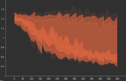
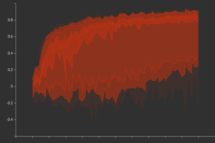
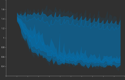
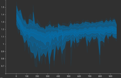
Utilising batch hard mining, the model demonstrated the ability to separate negative samples from the positives. At the commencement of training, the mean of Attraction Term was higher than the Repulsion Term. By the end of the training process, the model successfully minimised the Attraction Term from approximately $1.4\text{to}0.7$, while the Repulsion Term was consistently concentrated between $1.15\text{and}1.25$.

Attraction Term	Repulsion Term

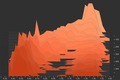
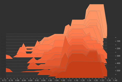
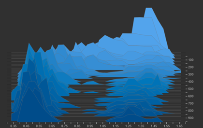
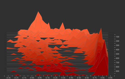
The histograms further illustrated these favourable dynamics; the distribution of the Repulsion Term remained concentrated on the right side of the axis, while the Attrasction Term distribution successfully shifted to the left. This increasing spatial separation the two density peaks provides clear visual evidence that the model learnt to distinguish between genuine signatures and forgeries, effectively widening the margin.

Attraction Term	Repulsion Term

When evaluated on the withheld test set, the model yielded a classification accuracy of $78.23\%$. This indicates that the system correctly identified signatures in approximately 78 out of every 100 instances, demonstrating acceptable performance for this specific evaluation context. The relatively high anchor-positive cosine similarity alongside a low anchor-negative cosine similarity confirms the model’s capacity to discern forgeries from genuine signatures. Furthermore, an analysis across the entire threshold range identified $0.667$ as the optimal threshold, at which point the misclassification rate was $21.77\%$.

Category	Metric / Score	Result
Performance	Accuracy	$78.23\%$
	True Positive Rate	$78.20\%$
	False Positive Rate	$21.80\%$
	AUC	$0.8607$
	EER	$21.77\%$
Similarity Score	Positive Score	$0.7784$
	Negative Score	$0.3611$

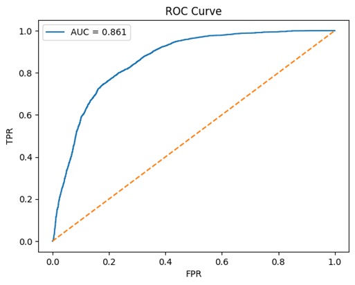
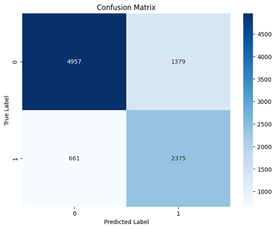
Hard mining produced smooth and globally consistent boundaries, as illustrated by the clean ROC curve. The curve yields an AUC of $0.8067$, suggesting that the embedding space learnt under hard triplet mining maintains a strong degree of class separability across varying thresholds. However, the confusion matrix reveals a more detailed picture; even at the optimal threshold, False Acceptance Rate remains relatively high ($\approx 21.8\%$). This indicates that a significant portion of skilled forgeries still resides within the acceptance margin of the genuine clusters.

These results demonstrate that while hard-negative mining successfully increases inter-class separation for the hardest violations, it does not guarantee robust generalisation across all variations of the same signature. Consequently, hard triplet mining alone may not suffice for real-world signature verification, necessitating further refinement or the integration of complementary strategies.

Semi Hard Triplet Mining

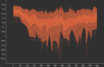
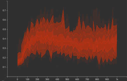
Under the batch semi-hard mining strategy, the model demonstrated a capacity to separate negative samples from positive. At the start of training, the Attraction and Repulsion Terms exhibited similar means, indicating an initial lack of discriminative structure in the embedding space. By the end of training, the mean Attraction Term was successfully reduced from $1.1$ to $\approx 0.7$, while the Repulsion Term stabilised between $1.1\text{and}1.2$.

Attraction Term	Repulsion Term

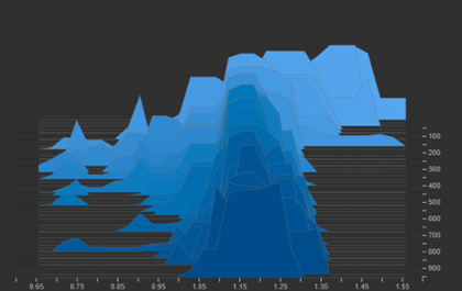
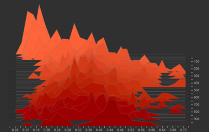
Visualisations via histograms confirmed these desired changes. The distribution of the Attraction term shifted to the left, indicating tightening clusters. Although the Repulsion Term appeared to shift towards the centre rather than staying on the right, this is a visual noise caused by the disproportionately high distances recorded during the start of the training. Nonetheless, the Repulsion Term shifted to a stable range, ensuring a consistent, clearly defined margin.

Attraction Term	Repulsion Term

Upon evaluation with the test set, the model achieved a Recall rate of $82.10\%$ and a False Positive Rate (FPR) of $17.90\%$. The high positive similarity scores and mid-range negative scores further validated the model’s ability to cluster positives and their variants. Finally, at the optimal decision threshold of $0.777$, the model yielded a Total Error Rate of $17.88\%$.

Category	Metric / Score	Result
Performance	Accuracy	$82.12\%$
	True Positive Rate	$82.10\%$
	False Positive Rate	$17.90\%$
	AUC	$0.9071$
	EER	$17.88\%$
Similarity Score	Positive Score	$0.8639$
	Negative Score	$0.4967$

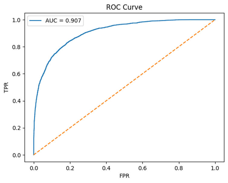
The ROC curve is smooth and clean with a high AUC score of 0.907. While the confusion matrix still indicates some leakage, especially skilled forgeries that manage to bypass the threshold, the overall pattern suggests that semi-hard mining produces a balanced embedding space. This strategy did not create a model that is overly sensitive to extreme outliers but rather one that focuses on samples that lie within the margin but not yet properly separated.

ROC Curve	Confusion Matrix

$L_{SC+}$

Unlike standard triplet loss, the l$L_{SC+}$ loss function utilises cosine similarity, effectively inverting the traditional distance-based intuition. In this architecture, the repulsion mechanism pushes hard negatives toward lower similarity values, while the explicit positive pull ensures that the attraction term increases, but only up to the specified margin. This prevents the cluster from collapsing into a single point while ensuring that positive clusters are not too sparse.

During training, the model exhibited the desired behaviour: a rising Attraction Term and a diminishing Repulsion Term. The histograms for the Repulsion Term were notably spread out, indicating that the model is complying with the intended behaviour of ignoring easy forgeries and aggressively pushing hard negatives.

Attraction Term	Repulsion Term

Attraction Term	Repulsion Term

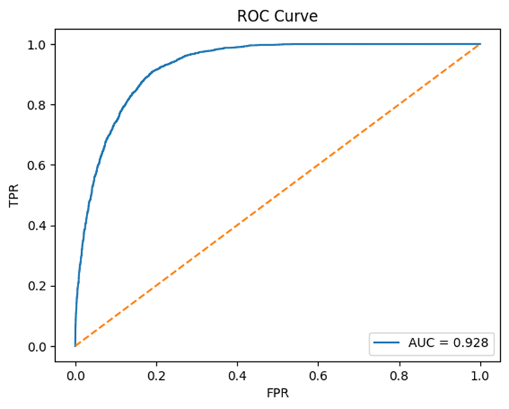
On the test set, the model yielded the most promising results, achieving a recall of $84.80\%$, a False Positive Rate of 15.20%, and an overall accuracy of $84.85\%$. At an optimal threshold of $0.725$, a respectable Equal Error Rate (EER) of $15.15\%$ was recorded.

Category	Metric / Score	Result
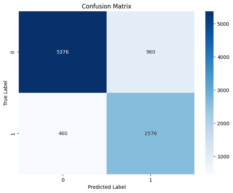
Performance	Accuracy	$84.85\%$
	True Positive Rate	$84.80\%$
	False Positive Rate	$15.20\%$
	AUC	$0.9284$
	EER	$15.15\%$
Similarity Score	Positive Score	$0.8444$
	Negative Score	$0.3644$

These metrics, alongside a superior AUC, point to a more discriminative embedding space than the triplet-based variants. The ROC curve shows smooth global separation, while the confusion matrix confirms consistent rejection of forgeries.

ROC Curve	Confusion Matrix

Performance and Evaluation

Quantitative Results

Amongst the three loss function, $L_{SC+}$ performed the best. While some overlap persists, it is miniimsed compared to the other strategies. This is likely to due its design of ignoring easy negatives, leading to closer, yet acceptable, distances. At the optimal threshold, this model yielded the lowest false acceptance of forgeries

Metric / Score	$L_{SC+}$ (0.725)	Semi-Hard Triplets (0.777)	Hard Triplet (0.667)
TPR	84.8%	82.1%	78.20%
FPR	15.2%	17.9%	21.80%
AUC	0.9284	0.9071	0.8607
Positive Score	0.8444	0.8639	0.7784
Negative Score	0.3644	0.4967	0.3611

Both positive and negative scores of $L_{SC+}$ fall between those of semi hard (0.8639) and hard mining (0.7784). While initially counterintuitive, this highlights a critial point: a hihger positive similarity doesn ot necessarily translate to better verification. What matters is the margin between potsitive and negative distributions is what a model should prioritise. $L_{SC+}$ achieves this by moderately enforcing intra-class compactness while consistently pushing hard negatives, creating more balanced clusters

The ability to decouple anchor-positive from anchor-negative pairs allows $L_{SC+}$ to receive independent gradient signals, ensuring continuous, informative updates regardless of triplet sampling quality. In contrast, the coupling effect in hard and semi-hard triplet mining causes imbalance gradients, leading to overlap. The smoother gradient dynamics of $L_{SC+}$ resulted in a more separable embedding space, improving discriminability across thresholds.

The operating threshold for $L_{SC+}$ falls between semi-hard and hard mining, reflecting a more balanced embedding distribution. By comparison, the lower threshold required by hard triplet ming reflects its tendency to over-compress positives, which shifts the negative distribution closer and increases false acceptance of forgeries.

Overall, the results indicate that $L_{SC+}$ produces more stable, generalizable, and discriminative embeddings. Despite not achieving the highest raw positive score, its improved separation of positive and negative distributions leads to superior AUC, TPR, FPR, and accuracy. This robustness arises from its decoupling of anchor-positive and anchor-negative contributions, which ensures continuous informative gradients and balanced embedding clusters.

Embedding Behaviour and Analysis

Across all loss functions, the models exhibited the desired behaviour: a leftward shift of anchor-positive distance and a lingering anchor-negative distance on the right

However, upon scrutiny, some nuances can be observed; there exist overlapping between the attraction and repulsion terms. The extent of this overlap and resulting stability varies significantly by strategy.

Hard triplet mining showed the most severe overlap between positive and negative distributions. This resulted in a higher rate of false predictions, even at the model’s optimal performance threshold. This aligned with the observation made by the authors of FaceNet ³, who noted that an over-focus on hard triplets often causes model collapse. The excessive penalty on hard negatives forced the model to over-compress anchor-positive pairs to compensate. This over-fitting to specific hard samples reduced the generalisability of the model to unseen signatures from the same signer. The imbalanced focus on hard negatives resulted in inconsistent separation of anchor-negative pairs, leaving some negatives closer to the anchor than desired.

Semi hard triplet mining exhibited less drastic overlap. This is likely due to its enforcement of separations based on $D_{ap}+\alpha$ rather than purely focusing on the hardest violations. However, this strategy can backfire when the threshold for forgeries falls within the $D_{ap}+\alpha$ range, where false predictions remain relatively high. Notably, its reduced emphasis on hard triplets leads to slightly more dispersed anchor-positive pairs, increasing robustness to intra-class variation by allowing natural differences in genuine signatures.

GradCAM

Source: https://github.com/jacobgil/pytorch-grad-cam

I will only highlight weird, edge cases since they’re the most interesting.

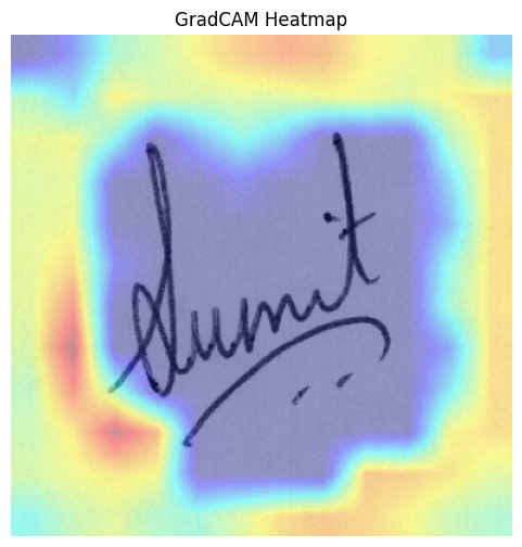
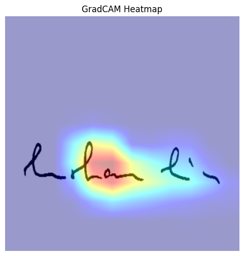
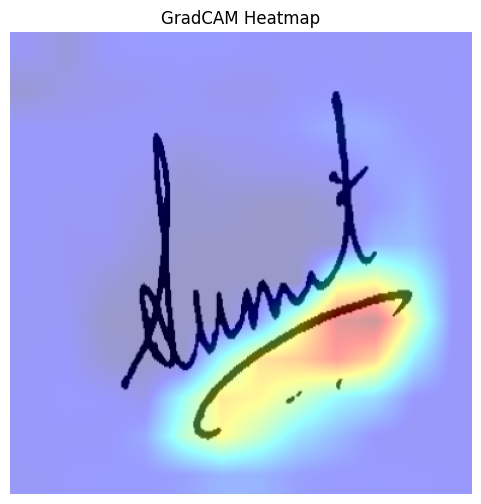
GradCAM is designed with classification models in mind, so the following interpretation may seem unorthodox.

Clever Hans Effect

As much as I wish it to be, my model is far from perfect. A significant issue present in a lot of models (both traditional and deep learning models) is the emergence of Clever Hans effect ⁸. In certain true positive instances, the model bypassed stroke characteristics in favour of spurious background features.

One plausible reason to this phenomenon is that the loss function forces discrimination in the embedding space, even when the model fails to discern meaningful biometric differences between certain pairs. As a result, the model resorted to minor background artefacts as proxy to manipulate distances, even if these artefacts have been largely mitigated via binarisation.

Fortunately, this is not consistent across every signature.

Signer 52	Signer 21

Implementation and Deployment

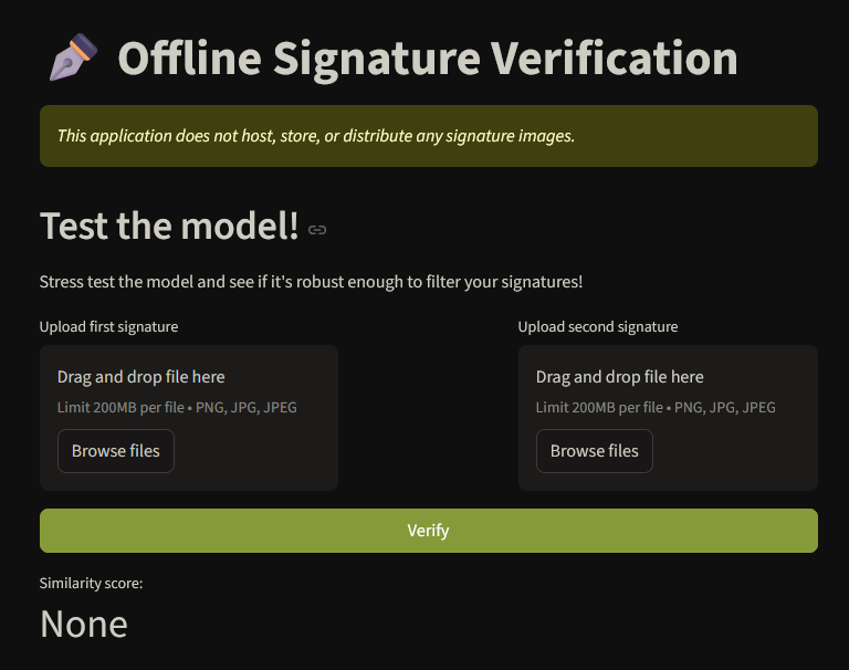
I’ve published the model onto hugging face and deployed it via streamlit.

Check it out here! Demo site

Previous version

I developed a backend API using Flask to handle verification requests.

A simple frontend is developed with React and a backend is developed using Flask microweb framework. I decided to implement a vector database using PostgreSQL with an open source plugin, pgvector ⁹. Finally, the entire system was containerised using Docker ¹⁰ for easy deployment and testing.

The webpage allows the user to insert a signature image along with the user’s details, and upon verification, the similarity score, confidence score, Euclidean distance, and the distance score will be calculated and displayed.

Future Developments

1. Extensive hyperparameter fine-tuning It usually results in diminishing return
2. Implementation and deployment It’s deployed to Streamlit
3. Try different datasets I’m making my own test dataset

Footnotes

1. EfficientNetV2 ↩ ↩² ↩³

2. Hard negative examples are hard, but useful ↩ ↩² ↩³ ↩⁴

3. FaceNet: A unified embedding for face recognition and clustering ↩ ↩²

4. Otsu’s Method ↩

5. CEDAR ↩

6. Pretrained models ↩

7. The book ↩

8. Couldn’t find a source that isn’t Wikipedia ↩

9. pgvector ↩

10. docker ↩