Data Source

The dataset includes lifestyle factors, health metrics, and demographic profile.

Gender	Age	Height(cm)	Weight(kg)	Family_history	Alcohol	Junk_food	Vege_day	Meals_day	Snack	Smoking	Water_intake(L)	Transportation	Exercise	TV	Income	Discipline	Cardiovascular_risk
Female	42	172.2	82.9	no	low	yes	3	3	Sometimes	no	2.72	car	3	rare	2081	no	medium
Female	19	175.3	80	yes	none	yes	2	1	Sometimes	no	2.65	bus	3	moderate	5551	no	medium
Female	43	158.3	81.9	yes	none	yes	3	1	Sometimes	no	1.89	car	1	rare	14046	no	high
Female	23	165	70	yes	low	no	2	1	Sometimes	no	2	bus	0	rare	9451	no	medium
Male	23	169	75	yes	low	yes	3	3	Sometimes	no	2.82	bus	1	often	17857	no	medium
Male	23	172	82	yes	low	yes	2	1	Sometimes	no	1	bus	1	moderate	3114	no	medium
Female	21	172	133.9	yes	low	yes	3	3	Sometimes	no	2.42	bus	2	moderate	8011	no	high
Male	21	172.5	82.3	yes	low	yes	2	2	Sometimes	no	2	bus	2	moderate	5838	no	medium
Female	19	165	82	yes	none	yes	3	3	Sometimes	no	1	bus	0	moderate	10029	no	high

Exploratory Data Analysis

WARNING

I don’t have much information over the dataset other than the data, so most of the analysis are speculations.

The dataset has 17 features, 1 label and 2100 rows:

row, column = cardio_df.shape
print(f"The number of rows: {row}\nThe number of columns: {column}\n")
 
cardio_df.info()

RangeIndex: 2100 entries, 0 to 2099
Data columns (total 18 columns):
 #   Column                  Non-Null Count  Dtype  
---  ------                  --------------  -----  
 0   Gender                  2100 non-null   object 
 1   Age                     2100 non-null   int64  
 2   Height(cm)              2100 non-null   float64
 3   Weight(kg)              2100 non-null   float64
 4   Family_history          2100 non-null   object 
 5   Alcohol                 2100 non-null   object 
 6   Junk_food               2100 non-null   object 
 7   Vege_day                2100 non-null   int64  
 8   Meals_day               2100 non-null   int64  
 9   Snack                   2100 non-null   object 
 10  Smoking                 2100 non-null   object 
 11  Water_intake(L)         2100 non-null   float64
 12  Transportation          2100 non-null   object 
 13  Exercise                2100 non-null   int64  
 14  TV                      2100 non-null   object 
 15  Income                  2100 non-null   int64  
 16  Discipline              2100 non-null   object 
 17  Cardiovascular_risk(y)  2100 non-null   object 
dtypes: float64(3), int64(5), object(10)
memory usage: 295.4+ KB

Information from the output above:

There are 17 features
There is no null values

Relevant features:

gender
age
height(cm)
weight(kg)
family_history
alcohol
junk_food
snack
smoking
transportation
exercise
tv
discipline

Height and weight are combined to calculate BMI, as individually they don’t provide much meaningful information.

Univariate Analysis

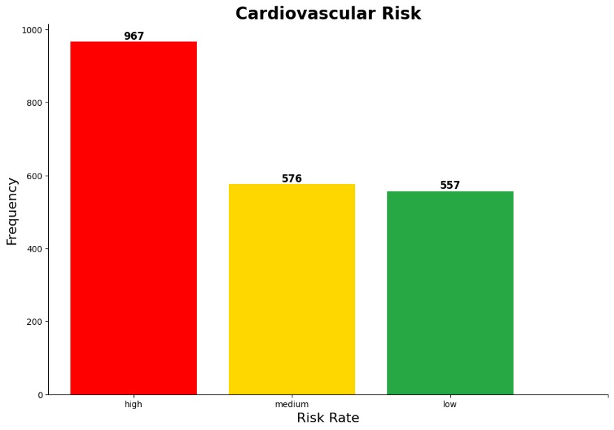
Cardiovascular Risk

Age, Weight, and Height

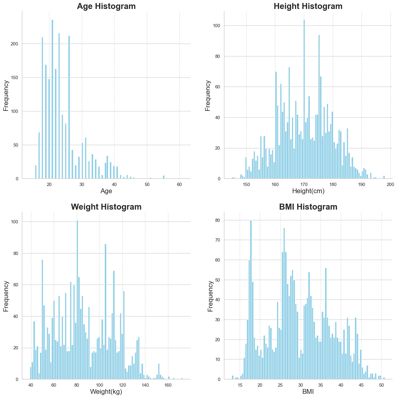
The age distribution is right-skewed, indicating that the demographic of the dataset is primarily teenagers and working adults. Based on the cardiovascular risk graph, this suggests that most individuals with a higher risk of cardiovascular disease are younger.

Finally, the BMI histogram denotes a multimodal distribution, as shown by the presence of multiple peaks. There are peaks between 15 and 20, between 25 and 30, and between 30 and 40, suggesting several underlying subpopulations or distinct clusters with different BMI ranges.

Lifestyle and Demographic

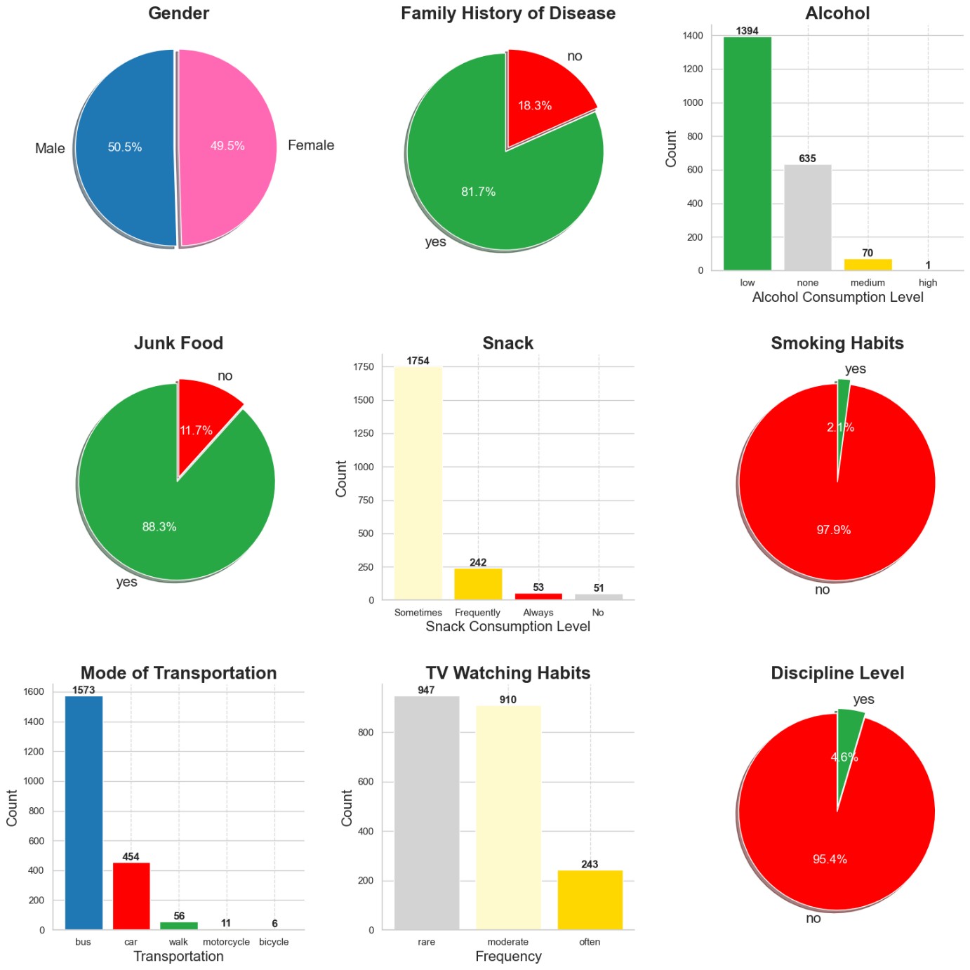
Both genders are evenly represented in the dataset, which may help minimise potential bias in the machine learning models and prevent them from skewing toward one gender .

The majority of individuals — 81.7% — have a family member with cardiovascular disease, while only 18.3% report no such family history. A family history of cardiovascular disease is shown to elevate the risk factor ¹². Despite the reported low levels of alcohol consumption, other contributing factors are likely driving the observed cardiovascular risk. There are arguments that low to moderate alcohol consumption is cardio-protective amongst apparently healthy individuals ³; however, this conclusion came from older studies which may had methodological issues, attenuating the strength of the conclusion. Nonetheless, modern research suggests that the risks of alcohol consumption outweigh any potential benefits ⁴.

In terms of performance, the large gap between the levels of consumption may introduce bias to the model. The large disparity between transportation via bus and via bicycle may suggest that the data was collected from urban areas where buses are a common mode of transportation, while cycling is less prevalent. This could also provide insights into the overall physical activity levels of the sample, as reliance on buses may correlate with lower physical activeness compared to cycling.

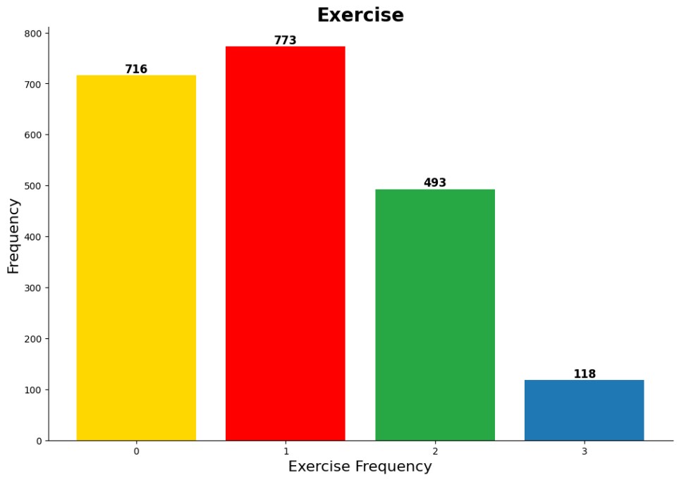
The majority of the sample reported engaging in little to no regular physical activity, a a factor known to elevate cardiovascular risk ⁵.

Bivariate Analysis

Age and Cardiovascular Risk Levels

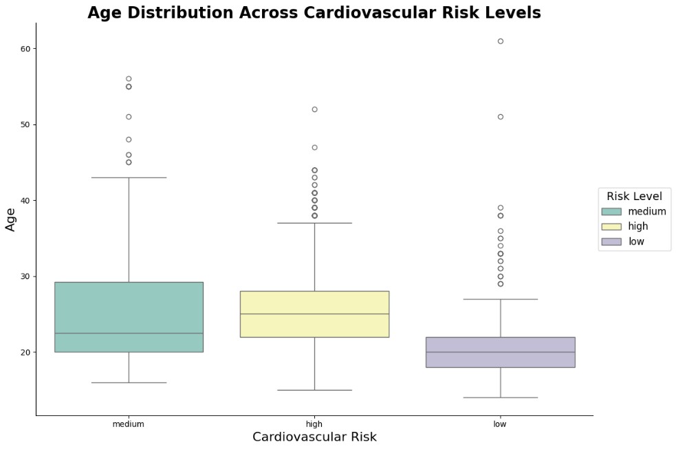
The boxplot for the low-risk category indicates that most individuals are relatively young, with a lower median age compared to other risk categories. The age range is narrow of ages, suggesting limited variability, although a few outliers extend into older age groups.

In contrast, the medium-risk category exhibits a wider age distribution, with the median age slightly higher than that of the low-risk group. The presence of several outliers, along with the broader spread, suggests greater diversity in age among individuals in this category.

BMI and Cardiovascular Risk

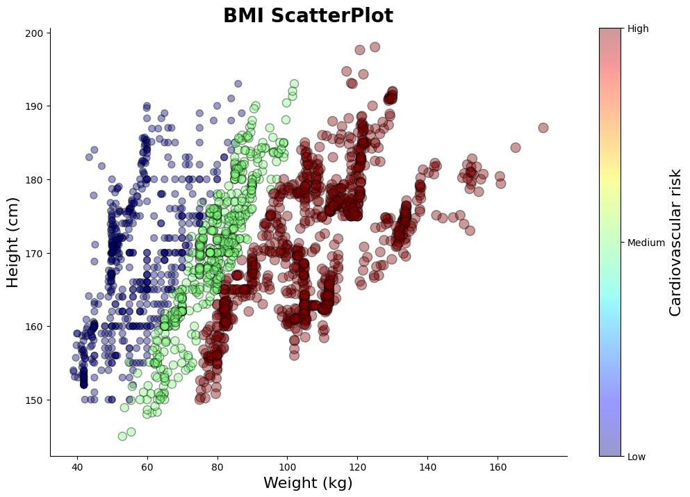
The scatter graph reveals a positive correlation between BMI and cardiovascular risk. Individuals with lower BMI tend to exhibit lower risk levels for cardiovascular diseases, whereas those with higher BMI appear to face elevated risk.

Gender and Cardiovascular Risk

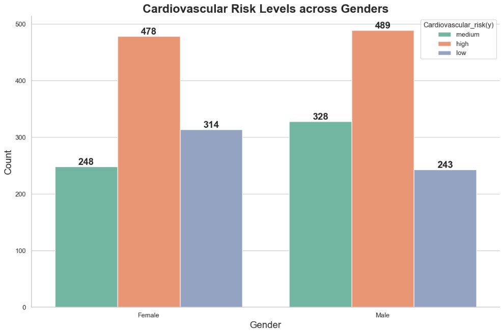
The graph indicates that the distribution of cardiovascular risk between the two genders is relatively even. Both females and males show the highest count in the high-risk category, with each reaching 500, suggesting that high cardiovascular risk is prevalent across both genders. However, the number of individuals in the medium-risk category is higher among males compared to females. Additionally, fewer males fall into the low-risk category than females.

Lifestyle and Cardiovascular Risk

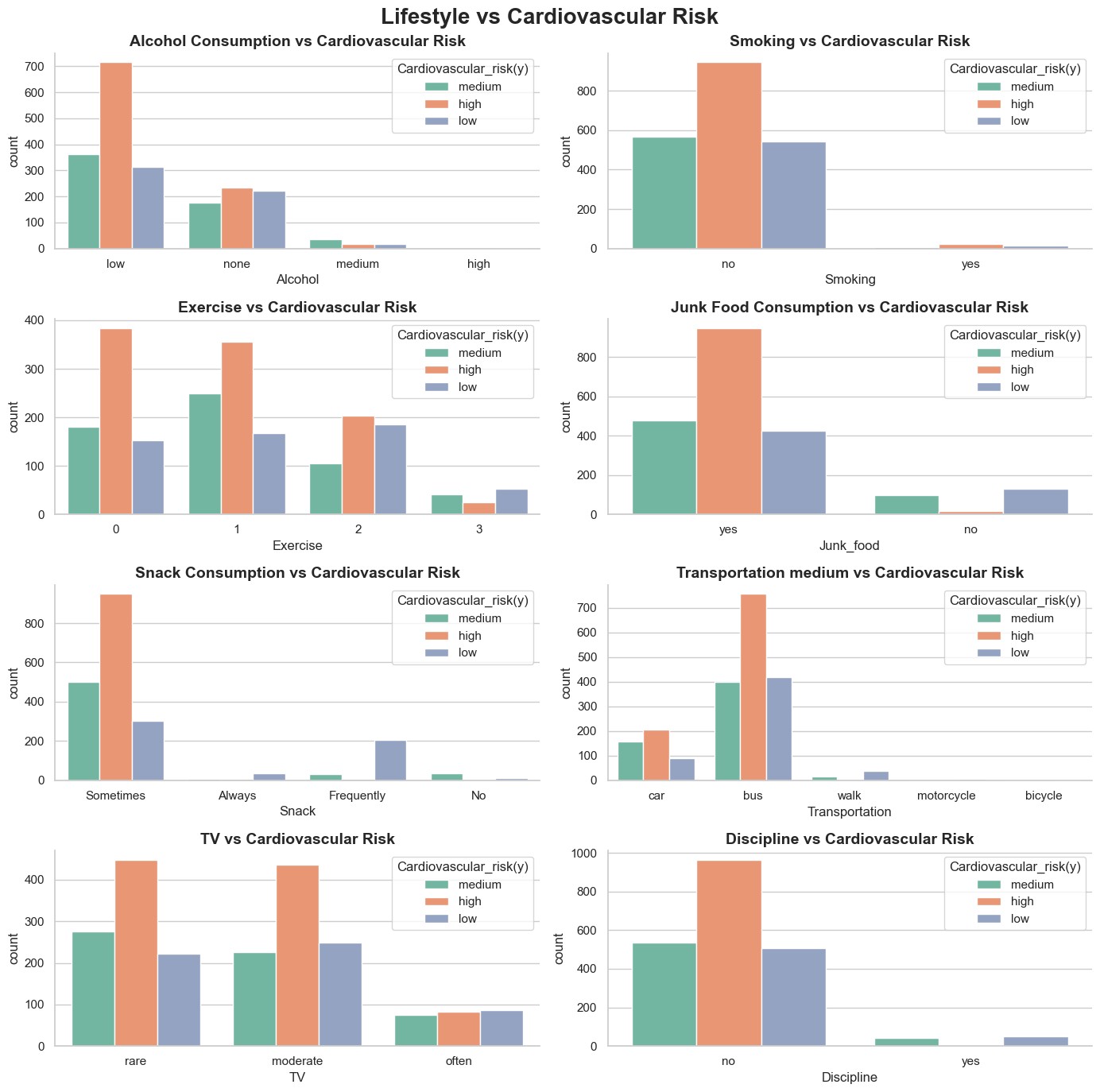
It can be observed that a significant portion of individuals who consume low volumes of alcohol exhibit higher cardiovascular risks, suggesting that other factors - such as physical activity and dietary habits - may play a more influential role.

A similar trend is seen with smoking status, snack consumption rate, and television viewing habits. The majority of individuals who do not smoke, occasionally indulge in snacks, and rarely watch television still fall into the high cardiovascular risk category, indicating that these behaviours alone do not fully account for cardiovascular health outcomes.

Individuals who do not engage in regular physical activity are more likely to fall into high cardiovascular risk categories compared to those who exercise consistently ⁵. Moreover, those who rely on passive transportation methods - such as driving or public transport - tend to have significantly higher cardiovascular risk than individuals who use active modes of transport like walking or cycling ⁶.

A large proportion of individuals who admit to regularly consuming junk food also fall into the high-risk category ⁷. Finally, individuals believe they lack personal discipline are more likely to be categorised as a high-risk compared to those who consider themselves disciplined.

Data Cleaning and Pre-processing

There are much better ways to handle skewed data - logging, Yeoh-Johnson, etc.

Due to the highly skewed distribution in numerical data such as age, height, weight, and exercise frequency, the dataset contains a significant number of outliers. Before proceeding with outlier removal, height and weight are first combined into the Body Mass Index (BMI), which provides a more meaningful metric for assessing body fat in relation to height and weight.

Removing outliers from height and weight independently before calculating BMI may lead to overlooking important interactions between these features. While weight and height values may appear extreme when observed in isolation, their combination in BMI could produce values that fall within a normal range. Therefore, deriving BMI before filtering outliers helps preserve the integrity of feature relationships and ensures a more accurate representation of physical health indicators.

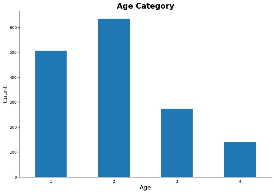
The age feature remains right-skewed, making discretisation a beneficial pre-processing step to ensure balanced representation across age groups.

Among the selected features, six contain nominal data and three contain ordinal data. Of the nominal features, 5 – gender, family, junk food, smoking, and discipline - will be pre-processed with LabelBinarizer, as they are binary and applying OneHotEncoder would introduce unnecessary complexity. The transportation feature, which contains more than two categories, will be encoded with OneHotEncoder.

For the ordinal features - alcohol consumption, television viewing, and snack frequency - OrdinalEncoder will be used to preserve their inherit order. Additionally, for improved model performance and interpretability, cardiovascular risk will also be encoded using OrdinalEncoder.

Methodology

Model Training

This is a supervised, offline, multi-class classification problem.

The models selected for evaluation are K-Nearest Neighbours, Extended Logistic Regression, and Random Forest. Model performance is assessed using the confusion matrix, precision, recall, F1 score, and the AUC-ROC curve, providing a comprehensive view of classification effectiveness.

K-Fold Cross Validation is employed, implemented manually through StratifiedKFold. This approach provides greater control over data splits and facilitates the measurement of specific performance metrics across consistent stratified folds, preserving the distribution of target classes in each fold.

K-Nearest Neighbours

K-NN performs well with relatively small datasets, such as the one used here with only 1, 900 rows. As a non-parametric algorithm, K-NN makes no assumptions about the underlying data distribution, making it versatile across various data types and distributions.

The number of neighbours considered plays an important role in model behavior:

A large value of k allows the algorithm to be more sensitive to the local structure, but increases the risk to overfit
A smaller value of k may improve generalisation, but could lead to underfitting if too few neighbours are used.

To determine proximity, distance metrics are applied. The three most common ones include:

Euclidean distance
Manhattan distance
Minkowski distance

Training the Model

K-fold cross validation result with default parameters:

Metrices	Value
Accuracy	0.9871
Precision	0.9875
Recall	0.9871
F1	0.9871

Metrics after training on the entire training set:

Metrices	Value
Accuracy	0.9961
Precision	0.9961
Recall	0.9961
F1	0.9961

Evaluation of Training Result

Classification report

Class	Precision	Recall	F1-Score	Support
Low	1.00	0.99	0.99	439
Medium	0.99	1.00	0.99	417
High	1.00	1.00	1.00	697
Accuracy	-	-	1.00	1553
Macro Avg	1.00	1.00	1.00	1553
Weighted Avg	1.00	1.00	1.00	1553

Confusion Matrix	Learning Curve

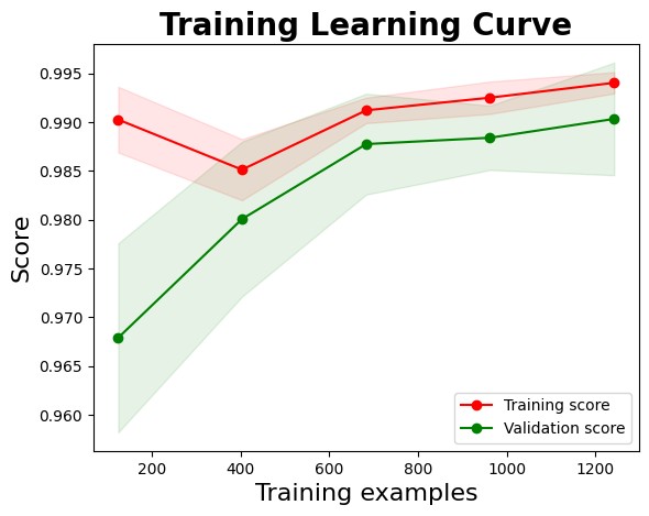The learning curve illustrates that the training score begins at a high level and remains largely stable, with only a slight initial dip before settling. This consistent performance may suggest some degree of overfitting. This consistent performance may suggest some degree of early overfitting. In contrast, the validation score starts noticeably lower but improves significantly as the number of training samples increases, reflecting better generalisation over time.

The narrowing gap between training and validation scores with increased data highlights improved model generalisation. As the model encounters more diverse samples, its ability to generalise beyond the training set strengthens, reducing overfitting and enhancing predictive reliability.

Logistic Regression

In the One-vs-Rest (OvR) approach, three separate binary logistic regression models are trained, each acting as a detector for a specific cardiovascular risk class: low risk, medium risk, and high risk. During classification, each model outputs a confidence score for its respective class, and the individual is assigned to the class with the highest predicted score among the three.

Training the Model

K-fold cross validation result with default parameters:

Metrices	Value
Accuracy	0.9852
Precision	0.9852
Recall	0.9852
F1	0.9852

Metrics after training on the entire training set:

Metrices	Value
Accuracy	0.9923
Precision	0.9923
Recall	0.9923
F1	0.9923

Evaluation of Training Result

Classification report

Class	Precision	Recall	F1-Score	Support
Low	0.99	0.99	0.99	439
Medium	0.99	0.98	0.99	417
High	1.00	1.00	1.00	696
Accuracy	-	-	0.99	1552
Macro Avg	0.99	0.99	0.99	1552
Weighted Avg	0.99	0.99	0.99	1552

Confusion Matrix	Learning Curve

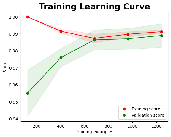Similar to the learning curve observed in the KNN model, this model initially exhibits signs of overfitting, with a very high training score early on. As more data is introduced, the training score slightly dips, reflecting reduced overfitting and a shift toward generalisable patterns. Meanwhile, the validation score begins substantially lower but improves steadily with increasing data, indicating enhanced generalisation.

Random Forest

Random forest is valuable for feature selection, as it ranks the relative importance of each input variable. This helps determine the features with the greatest impact on the prediction, making it useful for data analysis and model interpretation.

Training the Model

K-fold cross validation result with default parameters:

Metrices	Value
Accuracy	1.0
Precision	1.0
Recall	1.0
F1	1.0

Metrics after training on the entire training set:

Metrices	Value
Accuracy	1.0
Precision	1.0
Recall	1.0
F1	1.0

Although the K-Fold Cross Validation and overall training metrics appear perfect, this may be a sign that the model has overfitted; the model might have learnt noise or peculiarities in the data rather than generalisable patterns.

Evaluation of Training Result

Class	Precision	Recall	F1-Score	Support
Low	1.00	1.00	1.00	439
Medium	1.00	1.00	1.00	417
High	1.00	1.00	1.00	697
Accuracy	-	-	1.00	1553
Macro Avg	1.00	1.00	1.00	1553
Weighted Avg	1.00	1.00	1.00	1553

Confusion Matrix	Learning Curve

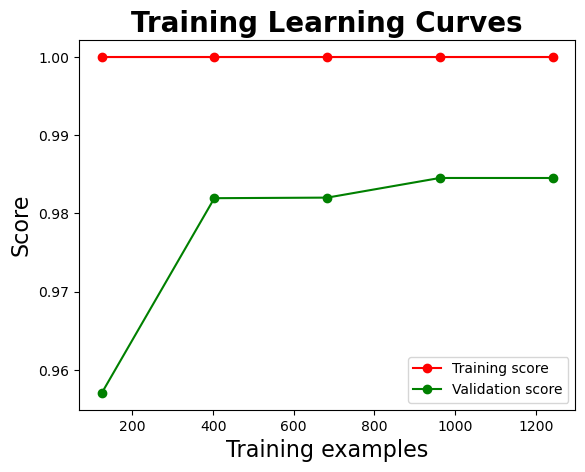Based on the confusion matrix, the Random Forest model produced a perfect training result, with zero misclassification across all three cardiovascular risk levels. While this may appear ideal, it raises concerns about potential overfitting.

The training score consistently remains at 1.0 across all sample size, while the validation score exhibits variation, reflecting the model’s fluctuating generalisation performance. Additionally, the absence of a shaded region between the training and validation learning curves suggests a minimal generalisation gap. Although this may seem encouraging, it could also indicate that the validation performance plateaus prematurely, possibly due to limitations in sample diversity or insufficient complexity in unseen cases.

Model Testing

K-Nearest Neighbours

Metrices	Value
Accuracy	0.9871
Precision	0.9877
Recall	0.9871
F1	0.9871

The performance of the model on unseen data is consistent with the performance on training data.

Confusion Matrix	AUC-ROC Curve

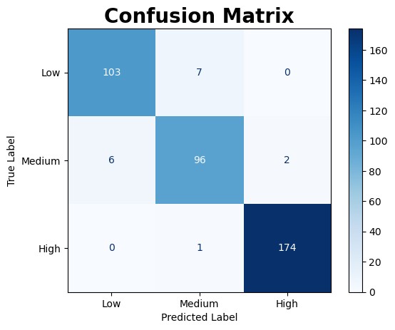
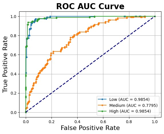
In comparison to the training confusion matrix, the validation performance shows minimal disparity. The model exhibits strong consistency, with only five misclassifications, all of which involve medium risk cases being incorrectly classified as low risk.

The AUC-ROC curve shows that the Area Under the Curve for each cardiovascular risk category consistently reaches 1.000, indicating that the model is highly effective at distinguishing between the three classes. The perfect AUC score for the high-risk category aligns with its flawless prediction performance in the confusion matrix, while only minor misclassifications are observed between the low and medium risk groups.

With the testing result closely matching the training result, this suggests that the model has generalised well without significant overfitting.

Overall, considering the classification metrics, confusion matrix, and AUC-ROC analysis, the model demonstrates strong performance and appears to be a suitable candidate for addressing the classification task.

Logistic Regression

Metrices	Value
Accuracy	0.9897
Precision	0.9897
Recall	0.9897
F1	0.9897

Confusion Matrix	AUC-ROC Curve

Comparing the two sets of metrics, the model’s performance on unseen data closely mirrors its performance on the training data, demonstrating consistent behaviour across both phases.

In the ROC AUC analysis, the model shows strong capability in distinguishing between the three cardiovascular risk categories. However, some misclassifications persist across all levels, indicating room for improvement in class separation.

Overall, based on the classification metrics, confusion matrix, and ROC AUC curve, the model appears to generalize well without significant overfitting, making it a strong candidate for addressing this classification problem

Random Forest

Metrices	Value
Accuracy	0.9897
Precision	0.9897
Recall	0.9897
F1	0.9897

Confusion Matrix	AUC-ROC Curve

While performance metrics declined slightly on unseen data, they still remained consistently high, indicating strong generalisation capabilities.

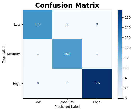
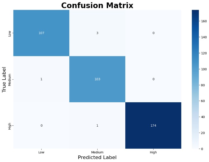
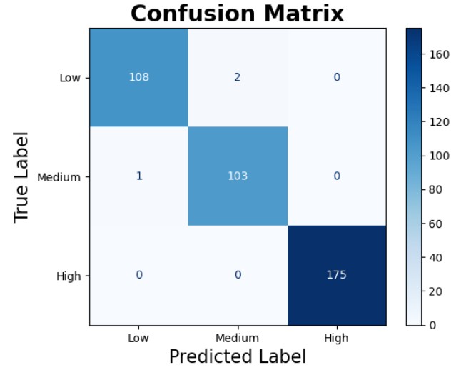
The confusion matrix for the test data shows that the model performs very well, albeit not perfectly, when applied to new samples. Specifically, 108 instances of low risk were correctly classified, with 2 misclassified as Medium and none as High. For the medium risk category, 103 instances were correctly predicted, while 1 low-risk instance misclassified. In the high-risk category, the model achieved perfect classification, correctly identifying all 175 instances with no misclassifications. While minor error exists in the low and medium categories, the overall performance remains robust.

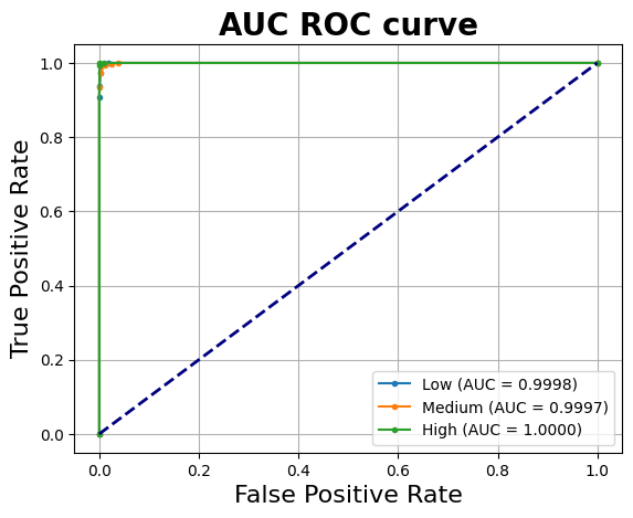
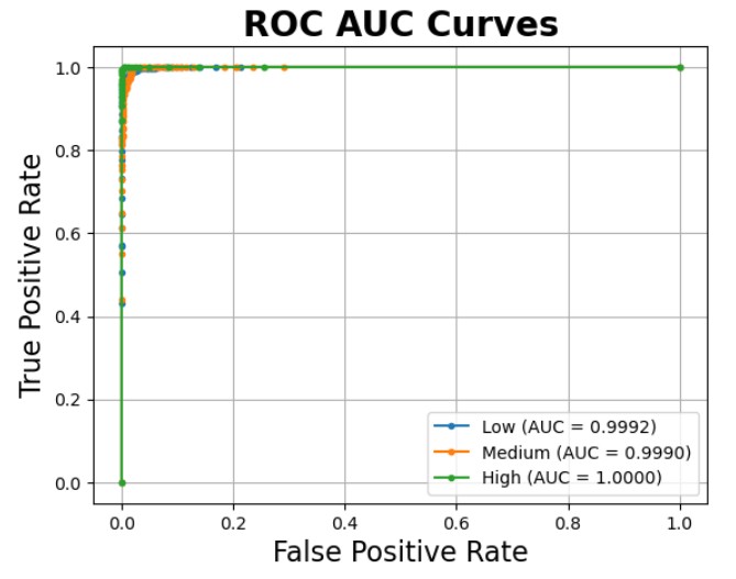
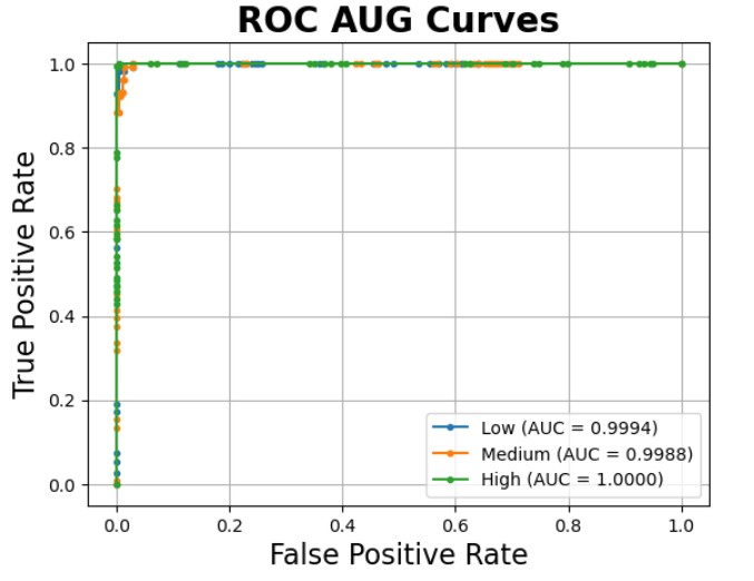
The ROC AUC curve demonstrates nearly perfect discrimination between the risk levels. The AUC values for low, medium, and high risk are 0.9992, 0.9990, and 1.0000, respectively. These near-ideal scores suggest excellent excellent predictive capabilities, with minimal false positives and high true positive rates across all classes.

Overall, the model shows strong generalisation and does not exhibit signs of overfitting, making it a promising candidate for addressing this classification task

Model Fine-Tuning

GridSearch is used for fine-tuning the model.

K-Nearest Neighbours

Two key hyperparameters—n_neighbors and the distance metric—are considered during model fine-tuning. Based on the results, the optimal KNN model employs the Manhattan distance metric and considers eight nearest neighbors for prediction.

Tuned Metrics:

Metrics (weighted)	Average
Accuracy	0.9871
Precision	0.9874
Recall	0.9871
$F_{1}$ Score	0.9872

F1 score improves slightly with the new, fine-tuned model but precision dips slightly.

Confusion Matrix	AUC-ROC Curve

According to the fine-tuned model, most misclassifications still occur within the medium-risk and low-risk categories, with one false negative and four false positives. Despite these minor errors, the ROC AUC curve shows a slight dip in the AUC for low-risk category, while the medium-risk category exhibits modest improvement.

Overall, the performance of the fine-tuned model improved, albeit marginally. The changes in classification accuracy and AUC suggest better calibration but indicate that further gains may require additional tuning or richer feature engineering.

Logistic Regression

During the fine-tuning stage, five key hyperparameters were considered for optimizing the logistic regression model:

regularization strength (C)
penalty
maximum iterations (max_iter)
solver options
class weight

Since the model is extended to One-vs-Rest (OvR) multiclass classification approach, only solvers compatible with OvR were selected. Given the relatively small dataset size of 1,900 samples, the sag and saga solvers were excluded, as they are better suited for larger datasets.

Solvers were fine-tuned separately, taking into account their support for specific penalty types:

liblinear can support both l1 and l2 penalties
lbfgs supports only l2.

The best-performing logistic regression model was found to use the following configuration:

C: 0.1
max_iter: 5000
penalty: l2
solver: lbfgs
class_weight: balanced

Metrics (weighted)	Average
Accuracy	0.989717
Precision	0.989708
Recall	0.989717
$F_{1}$ Score	0.989703

Confusion Matrix	AUC-ROC Curve

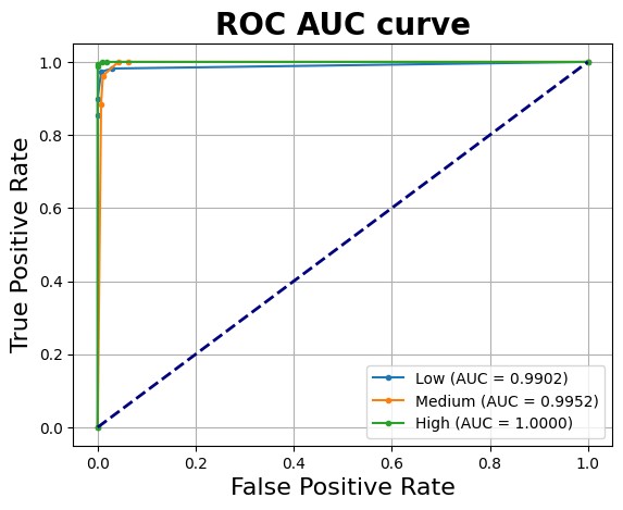
The fine-tuned confusion matrix closely resembles the testing confusion matrix, indicating consistent performance across evaluation stages. Based on the ROC AUC Curve, the model exhibits a slight improvement in its ability to differentiate between the three cardiovascular risk categories. However, the low-risk category continues to show the lowest AUC score among the three categories.

The optimal parameters for the alternative solver, liblinear, are:

C: 0.1
max_iter: 5000
penalty: l1
solver: liblinear
class_weight: balanced.

However, despite tuning, this configuration underperforms compared to the model trained using the lbfgs solver. The results suggest that lbfgs, combined with l2 regularization, yields better overall classification performance for this dataset.

Metrics (weighted)	Average
Accuracy	0.958869
Precision	0.958757
Recall	0.958869
$F_{1}$ Score	0.958804

Confusion Matrix	AUC-ROC Curve

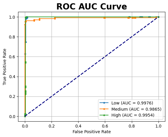
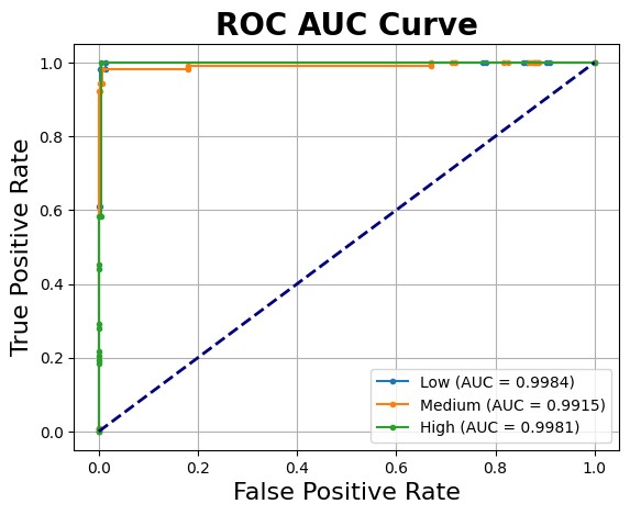
The model exhibits the greatest difficulty in distinguishing between the low and medium cardiovascular risk categories. This is reflected in the ROC AUC curve, which indicates that the model struggles more with predicting medium risk compared to low or high risk classifications.

Random Forest

The fine-tuning process involved evaluating 576 unique parameter combinations through 5-fold cross-validation, resulting in a total of 2,880 individual model fits.

The grid search explored parameters:

max_depth
max_features
min_samples_leaf
min_samples_split
n_estimators

Metrics (weighted)	Average
Accuracy	0.992288
Precision	0.992313
Recall	0.992288
$F_{1}$ Score	0.992289

Confusion Matrix	AUC-ROC Curve

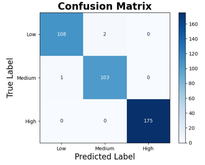
The fine-tuned confusion matrix remains identical to the original testing confusion matrix, underscoring consistent classification behaviour across both evaluations. The ROC AUC scores for the fine-tuned model indicate near-perfect performance, with only minor variations observed between the two scenarios.

The AUC for the low-risk category slightly increased from 0.9992 to 0.9994
The AUC for the medium-risk category decreased slightly from 0.9990 to 0.9988
The AUC for the high-risk category remained perfect at 1.0000

These results reflect a high level of reliability and generalisation, with the fine-tuned model maintaining strong predictive power across all categories.

Results and Findings

Using the fine-tuned version of the each model,

Models/ Metrices	K-NN	Logistic Regression (solvers)		Random Forest
		`liblinear` with `l1` penalty	`lbfgs` with `l2` penalty
Recall (weighted)	0.987147	0.958869	0.989717	0.992288
Precision (weighted)	0.987387	0.958757	0.989708	0.992313
F1 Score (weighted)	0.987187	0.958804	0.989703	0.992289

Based on the evaluation metrics, the Random Forest model delivers the best overall performance, consistently achieving the highest scores across all categories. It is followed by Logistic Regression model using the lbfgs solver while K-Nearest Neighbours (K-NN) comes in last. The Logistic Regression model with the “liblinear” solver performs the worst amongst the four, although it still records scores above 0.9 across most metrices.

According to the confusion matrices, Random Forest makes the fewest misclassifications when predicting cardiovascular risk levels, whereas the liblinear-based logistic regression model exhibits the most errors. Despite their differences, all models share a common challenge: most misclassifications occur between the low-risk and medium-risk categories, while the high-risk category is consistently predicted with high accuracy.

This trend can likely be attributed to the imbalanced distribution of risk levels in the dataset, where the high-risk category dominates, potentially leading to reduced performance on the minority classes. This imbalance may also explain why the liblinear solver, known to be more sensitive to class distribution, performs poorly in comparison.

Feature Importance

According to random forest,

Feature	Importance
BMI	0.722390
Snack	0.073774
Family_history	0.066922
Age_category	0.036632
Junk_food	0.017905
Exercise	0.014685
Alcohol	0.012645
TV	0.010880
Gender	0.010778
Transportation_bus	0.008732
Discipline	0.008573
Transportation_car	0.007792
Transportation_walk	0.004583
Smoking	0.003164
Transportation_motorcycle	0.000376
Transportation_bicycle	0.000170

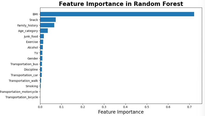
Body Mass Index (BMI) emerges as the most influential feature in predicting cardiovascular risk, with an importance score approaching 0.75. This indicates that BMI plays a dominant role in the model’s decision-making process. In contrast, the remaining features contribute significantly less to the prediction, suggesting that their impact on the model’s performance is relatively minor.

The prominence of BMI may reflect its strong correlation with cardiovascular outcomes, reinforcing its utility as a primary screening indicator in health-related classification tasks.

🥔

Table of Contents

Cardiovascular Risk Analysis

Table of Contents

Data Source

Exploratory Data Analysis